Demystifying Robotic Foundational Models: Pi0

The field of robotic foundation models is evolving rapidly. In just the past year or so, we've seen significant developments, arguably progressing from models like π₀ towards systems like Google's Gemini-Robotics and NVIDIA's Project GR00T. This is the first article in the series focused on Pi0, next we will look at Gemini robotics and Groot N1. Let's dive into π₀ to understand its architecture and training, which provides valuable context for appreciating later advancements.
We also have an accompanying video, just in case you prefer that more to the blog.

π₀

The Model Architecture

A common starting point for many recent robotics models is a pre-trained Vision-Language Model (VLM). This makes sense because VLMs, trained on vast amounts of internet data, already possess a strong semantic understanding of language and visual concepts – capabilities highly relevant for interpreting robot tasks and environments.

The π₀ model itself is relatively lightweight at ~3.3 billion parameters. It uses Google's PaliGemma (a 3B parameter VLM) as its foundation, which in turn was based on the Gemma architecture.
π₀ adapts this VLM backbone for robot control, effectively turning it from a VLM into a Vision-Language-Action (VLA) model.

This adaptation involves "extending" PaliGemma by adding a new component: the Action Expert (~300M parameters). This expert has its own set of weights, separate from the main VLM backbone. Inspired by the Transfusion architecture, the π₀ model, despite having these distinct weight sets, functions somewhat like a single unified transformer trained with different objectives for different types of outputs.

• Action Expert & Flow Matching: Since robot actions (like joint angles or end-effector movements) are continuous values, predicting them directly can be tricky. π₀ tackles this using Conditional Flow Matching. The Action Expert is trained specifically with a Flow Matching loss (essentially a Mean Squared Error between predicted and target vector fields) to learn how to generate realistic, continuous action sequences. We'll unpack this more below.   
• VLM Backbone & Language/Vision: The original PaliGemma backbone was trained using standard VLM objectives, likely involving cross-entropy loss for predicting text tokens and contrastive losses for aligning vision and language. While π₀'s robotics fine-tuning focuses on the flow matching loss for actions, the backbone retains its pre-trained ability to process images and language commands.   

A key output is action chunking. The Action Expert, using flow matching, predicts a sequence of H future actions (At​) at once (in the paper, H=50). This chunk represents the predicted robot movements for the next H control steps. Predicting chunks rather than single steps can be beneficial for executing smooth, high-frequency (up to 50Hz control loops mentioned ), and potentially long-horizon tasks.

How Information Flows: MoE Analogy & Attention

You can think of the architecture as a simplified Mixture of Experts (MoE) with two specialists: 

1. The VLM Expert (PaliGemma): Processes image and language tokens.
2. The Action Expert: Processes robot state tokens and the noisy action tokens used during flow matching training/inference.

These experts interact implicitly through the transformer's self-attention mechanism, allowing information to be shared. The flow of attention is carefully controlled using a block-wise causal attention mask:   

• Block 1: Images & Language Prompt: These tokens attend fully to each other but cannot attend to future blocks (state/actions). This helps preserve the VLM's pre-trained knowledge without being overly influenced by the robotics-specific inputs it wasn't originally trained on. The VLM's role here is to understand the scene and the command.   
• Block 2: Robot State (qt​): This token (representing current joint angles, etc.) attends to Block 1 (images/language). It cannot attend to Block 3 (actions). This is an efficiency trick: since the robot state doesn't change during the multiple steps of action inference, its attention keys/values can be calculated once and cached.   
• Block 3: Noisy Actions (Atτ​): These action tokens attend fully to each other (bidirectional attention within the chunk) and to Block 1 (images/language) and Block 2 (robot state). This allows the Action Expert to condition the predicted action sequence (vθ​) on the full context: the visual scene, the language command, and the robot's current physical configuration.   

Essentially, the model aims to predict a probability distribution over possible action chunks conditioned on the observations: p(At​∣Ot​).   

Observations (Ot​): For a given time step t, the observation Ot​ consists of:
 Ot = [Image_1, ..., Image_n, language_command, robot_state_qt] 

• Images: Multiple RGB camera views (e.g., wrist cams, third-person cams). The number varies depending on the robot setup. Missing image slots are masked out.   
• Language Command: Can range from high-level task descriptions (e.g., "fold the shirt" ) to more granular instructions. During pre-training, fine-grained text annotations for ~2-second trajectory segments were also used.   
• Robot State (qt​): A vector representing the robot's configuration, typically joint angles.   

If you are using LeRobot, this is how the data would look like for so100 arm:

data = LeRobotDataset(repo)

frame1 = data[0]
im_t_1 = frame1['observation.images.phone']
im_t_2 = frame1['observation.images.laptop']
l_1 = frame1['task']
q_1 = frame1['observation.state']
a_1 = frame1['action']

O_1 = [im_t_1, im_t_2, l_1, q_1]
im_1 = tensor_to_pil(reorder_tensor_dimensions(im_t_1))
im_2 = tensor_to_pil(reorder_tensor_dimensions(im_t_2))
display_images(im_1, im_2)
print("language_instruction: ", l_1)
print("Robot state, that joint angles for the motors: ", q_1)
print("Robot action: ", a_1)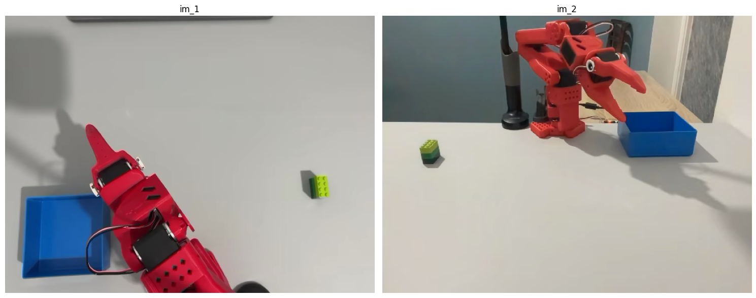

language_instruction: Grasp a lego block and put it in the bin.
Robot state, that joint angles for the motors: tensor([-32.0801, 166.0254, 162.1582, 40.2539, 6.0645, 31.1373])
Robot action: tensor([ 1.7578, 188.4375, 177.3633, 54.7559, -7.5586, 0.0000])

Flow Matching Deep Dive

The a math here might look intimidating, but its just an illusion; stay with me. We will break down the math to code and then it is plain old programming.
You can also follow along with this jupyter notebook.

• Goal Recap: Predict a chunk of H=50 future actions At​=[at​,...,at+H−1​] based on observation Ot​.   
• The Continuous Challenge: Robot actions are vectors of continuous numbers. Simply predicting the mean action (regression) might fail for complex tasks where multiple valid motions exist, or where high precision is needed.
• Flow Matching Idea: Learn a vector field vθ​ that tells us how to step-by-step transform simple noise into a valid action sequence matching the current observation.   

Training Phase:

1. Get Ground Truth: Take a real action chunk At​ from the dataset.
2. Sample Noise Level: Pick a "time" τ between 0 and 1, usually biased towards lower values (more noise) using a specific distribution (shifted Beta).   
3. Add Noise: Create a noisy version Atτ​ = τAt ​+ (1−τ)ϵ, where ϵ is random Gaussian noise N(0,I).

 # Sample tau (0 <= tau <= s < 1)
tau = sample_flow_timestep_tau()

# Sample noise
epsilon_noise = np.random.randn(ACTION_HORIZON, ACTION_DIM) 
noisy_actions_At_tau = tau * true_actions_At + (1.0 - tau) * epsilon_noise

4. Define Target: The "ideal" direction to step from the noisy action Atτ​ towards the true action At​ is given by the target vector field u = ϵ−At​. This is what we want our model to predict
5. Predict & Calculate Loss: Feed the noisy action Atτ​, the timestep τ, and the observation ot​ into the model (Action Expert) to get its predicted vector field vθ. Calculate the difference (MSE loss) between the prediction vθ​ and the target u. Use this loss to update the model's weights.

# Compute target vector field: u = epsilon - At
target_vector_field_u = epsilon_noise - true_actions_At

predicted_vector_field_v = model.predict(noisy_actions_At_tau, tau, observation_context)

# Calculate the loss (e.g., Mean Squared Error)
# Loss = || v_theta(At_tau, ot) - u(At_tau | At) ||^2
loss = np.mean((predicted_vector_field_v - target_vector_field_u)**2)

loss.backward() -> update weights

Action Generation (Inference) Phase:

1. Start with Noise: Generate a random action chunk At0​∼N(0,I). This is pure noise at τ=0.

# Start with random noise At0 ~ N(0, I)
current_actions_At_tau = np.random.randn(ACTION_HORIZON, ACTION_DIM)
current_tau = 0.0

2. Iterative Denoising: Use the trained model's predicted vector field vθ​ to take small steps from noise towards a valid action. Apply the Forward Euler integration rule repeatedly: Atτ+δ​=Atτ​+δvθ​(Atτ​, Ot​)

# Loop N times (e.g., N=10)
for step in range(NUM_INTEGRATION_STEPS):
       predicted_vector_field_v = model.predict(current_actions_At_tau, current_tau, observation_context) 
       
# Apply Euler step: At^{\tau+delta} = At^tau + delta * v_theta(At^tau, ot)
   current_actions_At_tau = current_actions_At_tau + DELTA * predicted_vector_field_v
   current_tau += DELTA

3. Final Prediction: After N steps (e.g., 10 in the paper ), the resulting action chunk At1​ is considered the model's prediction.   

Flow Matching Nuances: Tau Sampling and the Target Vector Field u

While the core idea of Flow Matching is elegant, the effectiveness often lies in the details of its implementation. Two important nuances in the π₀ model are the specific strategy for sampling the noise level (tau) during training and the precise definition of the target vector field (u) the model learns to predict.

Why a Special Tau Sampling Strategy? During training, we need to create noisy versions of our true actions At​ using the formula Atτ​=τAt​+(1−τ)ϵ. The variable τ∈[0,1] controls the noise level. A simple approach is to sample τ uniformly. However, the π₀ authors hypothesized that for robotics, accurately predicting actions under high uncertainty (high noise, τ≈0) is particularly challenging and crucial. Predicting the expected action E[At​∣Ot​] given an observation Ot​ is non-trivial, unlike perhaps predicting the mean of pixels in image generation.  

To focus the model's learning capacity on these difficult, high-noise scenarios, they devised a non-uniform sampling strategy. They use a transformation based on the Beta distribution (specifically Beta(1.5, 1.0)).   

1. A sample is drawn from Beta(1.5, 1.0), which tends to produce values closer to 1.
2. This sample is flipped (1 - sample), resulting in values skewed towards 0.
3. The result is scaled by a cutoff factor TAU_CUTOFF_S = 0.999, slightly limiting the maximum tau sampled.

This engineered distribution ensures that tau values closer to 0 are sampled more frequently during training (as visualized in the paper's Figure 14 ). The cutoff near 1 avoids spending training time on near-identity predictions where noise is minimal. This forces the model to get better at the hard task of determining the correct action direction even when starting from very noisy states.   

Understanding the Target Vector Field u:The heart of Flow Matching training is teaching the model vθ​ to predict a target vector field, denoted as u. Given the noisy action Atτ​ = τAt ​+ (1−τ)ϵ,
the target is defined as: u (Atτ∣At​) = ϵ − At​   

This u is the ground truth vector that the model's output vθ​(Atτ​,ot​) aims to match. The Flow Matching loss L(θ) directly minimizes the squared difference between vθ​ and u. Essentially, the model learns a mapping: "For this noisy input Atτ​ at this noise level τ, given observation Ot​, the ideal 'correction' vector you should point towards is u=ϵ−At​."   

Connecting Training Target (u) to Inference ("Moving in the Direction")
How does learning to predict u help generate actions during inference? The inference process uses the Euler integration step: Atτ+δ​=Atτ​+δvθ​(Atτ​,Ot​)   

Here, Atτ​ is the current action estimate (starting from noise At0​). The model predicts the vector vθ​ (its learned approximation of u). The formula then updates the current estimate by taking a small step (δ) in the multi-dimensional direction specified by the predicted vector vθ​.

"Moving in the direction" precisely means performing this update: adding the model's predicted vector vθ​ (scaled by δ) to the current position Atτ​. Although u was defined relative to the noise ϵ and true action At​ during training, the trained model vθ​ now implicitly encodes the learned dynamics. By iteratively applying these small steps guided by vθ​, the inference process follows the learned 'flow' from the initial random noise towards a realistic action chunk At1​ consistent with the observation Ot​.

Here is the accompanying code to better see a programmatic breakdown of the flow matching.

Why Flow Matching is Neat: It provides a structured way to model complex continuous distributions, potentially capturing multiple valid ways to perform an action (multi-modality) better than simple regression. It integrates nicely with transformers and enables generating these high-frequency action chunks needed for fluid robot control.

Data & Training Recipe

Alright, enough math for a bit. How is this model actually trained? The π₀ paper emphasizes a two-stage recipe, reminiscent of large language model training: pre-training followed by post-training (fine-tuning).   

• Pre-training Data: The foundation is built using a massive dataset – over 10,000 hours – combining Physical Intelligence's own data collected across 7 robot types and 68 tasks with public datasets like Open X-Embodiment (OXE). This data covers diverse robots (single-arm, dual-arm, mobile manipulators)and tasks.   
• Pre-training Goal: This phase aims for broad generalization. The data might be "crude" or less consistent ("lower quality" ) compared to specialized datasets, but its diversity is key. It teaches the model a wide range of basic physical interactions and, importantly, how to potentially recover from errors or handle unexpected situations, as varied behaviors are more likely present.   
• Data Weighting: To prevent tasks with vastly more data (like laundry folding, apparently!) from dominating the learning process, the data from different task-robot combinations is weighted during sampling.
• Post-training (Fine-tuning): After pre-training, the generalist model is fine-tuned on smaller, high-quality, task-specific datasets. This phase focuses on achieving skill – performing the target task efficiently, robustly, and fluently. The amount of fine-tuning data varies significantly: from ~5 hours for simpler adaptations to 100+ hours for highly complex tasks like mobile laundry folding.

HYPE Check: Even with this sophisticated approach and massive pre-training data, achieving high performance on complex tasks still requires significant fine-tuning data (tens or hundreds of hours) per task. This underscores that while progress is impressive, creating truly general-purpose robots capable of handling countless household chores or elder care autonomously is still a very challenging long-term goal. It's important to temper the hype sometimes seen in media or startup pitches. We're making strides, but general-purpose embodied AGI is not right around the corner.